In our previous installments we implemented two of the most well-known self-balancing binary search trees: AVL and Red-black trees.
We had a few classes on AVL trees in our basic data structures & algorithms class back in college, which made its implementation far less of a challenge than the Red-black tree. So besides the fundamental guidance of CLRS I had to do quite some googling to get it working. While googling I noticed there were quite a lot of questions about which (AVL or RB) tree was “better” in some sense, be it insertion, search time, deletion time, etc. Most textbooks and articles dismiss this question just by stating the factor differences in either trees’ worst case heights, as we briefly mentioned in the past installment. If you’re anything like me, however, you’ll want to see some comparisons where the trees are actually tested. So I decided to do some simple benchmarking to test those theoretical worst-cases. Here’s what I found out.
First off, we need at least two cases: worst and average case. As we know from the previous installments, the worst possible case for BST insertion is when you are inserting continuously increasing or decreasing values, e.g. 1, 2, 3, 4, … . In this case, a pure BST would behave exactly like a (doubly) linked list, while self-balancing trees should should spread out node distribution. The worst possible searches would be the top or bottom values, i.e. those close to the end of the “list”: a pure BST would have to traverse the entire list (n time), while self-balancing trees should enjoy a $latex k~log(n)$ time with some factor k.
What would an “average case” look like? Hard to say; depend on what is average for your application. It might just be the case that sequences are the average case. Since we can’t define a “universal” average case and for the sake of simplicity, we will define the average case as a sequence of random numbers drawn from C’s rand() function (one might argue that this is actually the “best” case since on the long run the BST will “naturally” become quite reasonably balanced, but let’s not get picky about terminology).
:————————-:|:————————-:
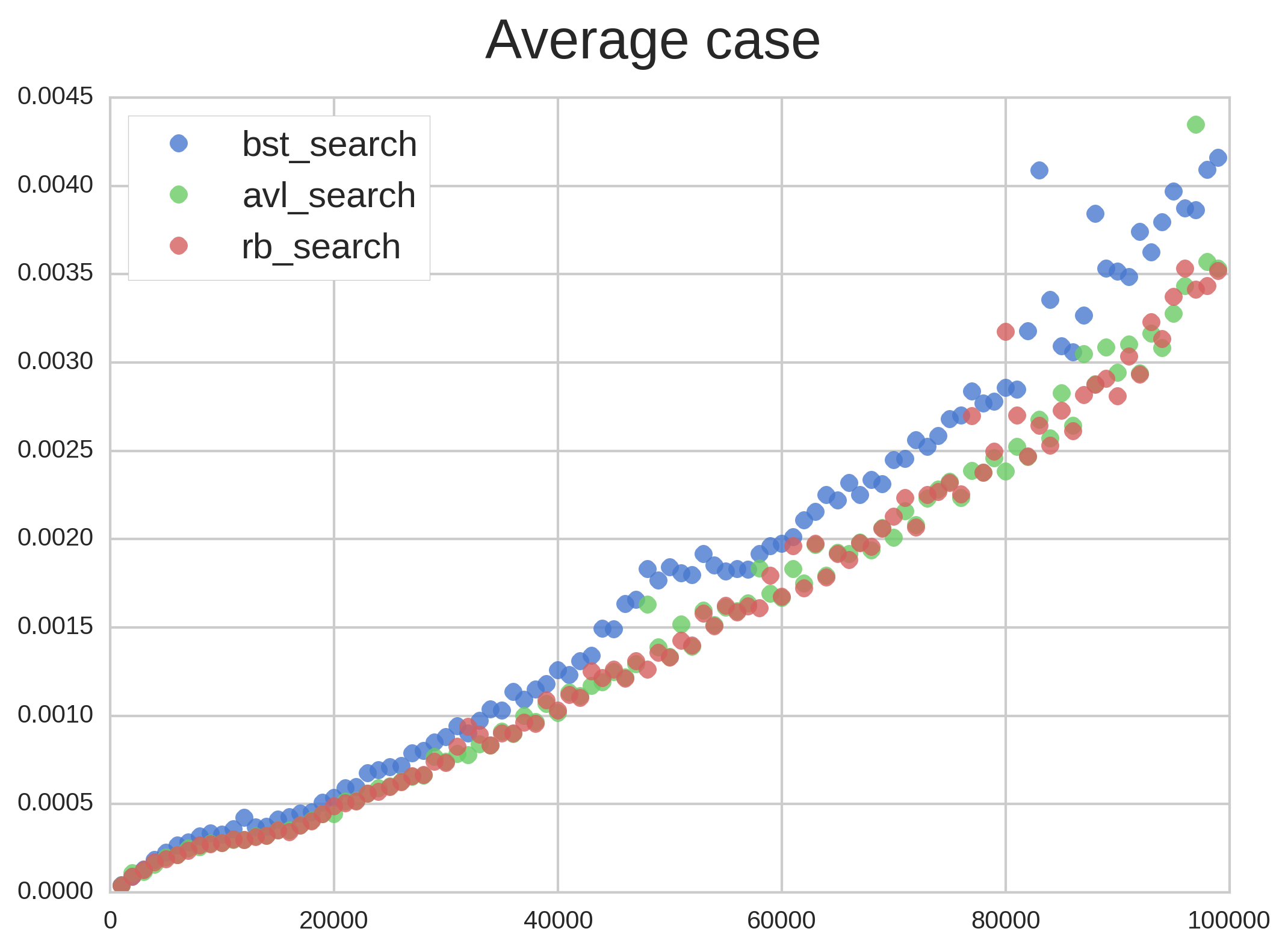
Figure 1
Benchmarking is done as follows: x values are inserted into the tree (x up to 100k in 1k steps), and then using the same tree we search for the bottom $latex frac{x}{10}$ values in the tree, so if x = 10k we will search for the 1k lowest values.
In Figure 1 we have insertion and search times for the average case. As we predicted, search times are basically the same for all 3 trees, with the unbalanced BST taking slightly more time than Red-black and AVL. The difference is small but seems to increase a bit as more elements are added. Insertion took significantly longer in the AVL tree than the other two, most likely due to all the rotations AVL needs to do. Red-black performed slightly better than BST. All in all, the 3 trees performed very similarly.
Now let’s see in Figure 2 how the trees perform in our worst-case scenario:
:————————-:|:————————-:
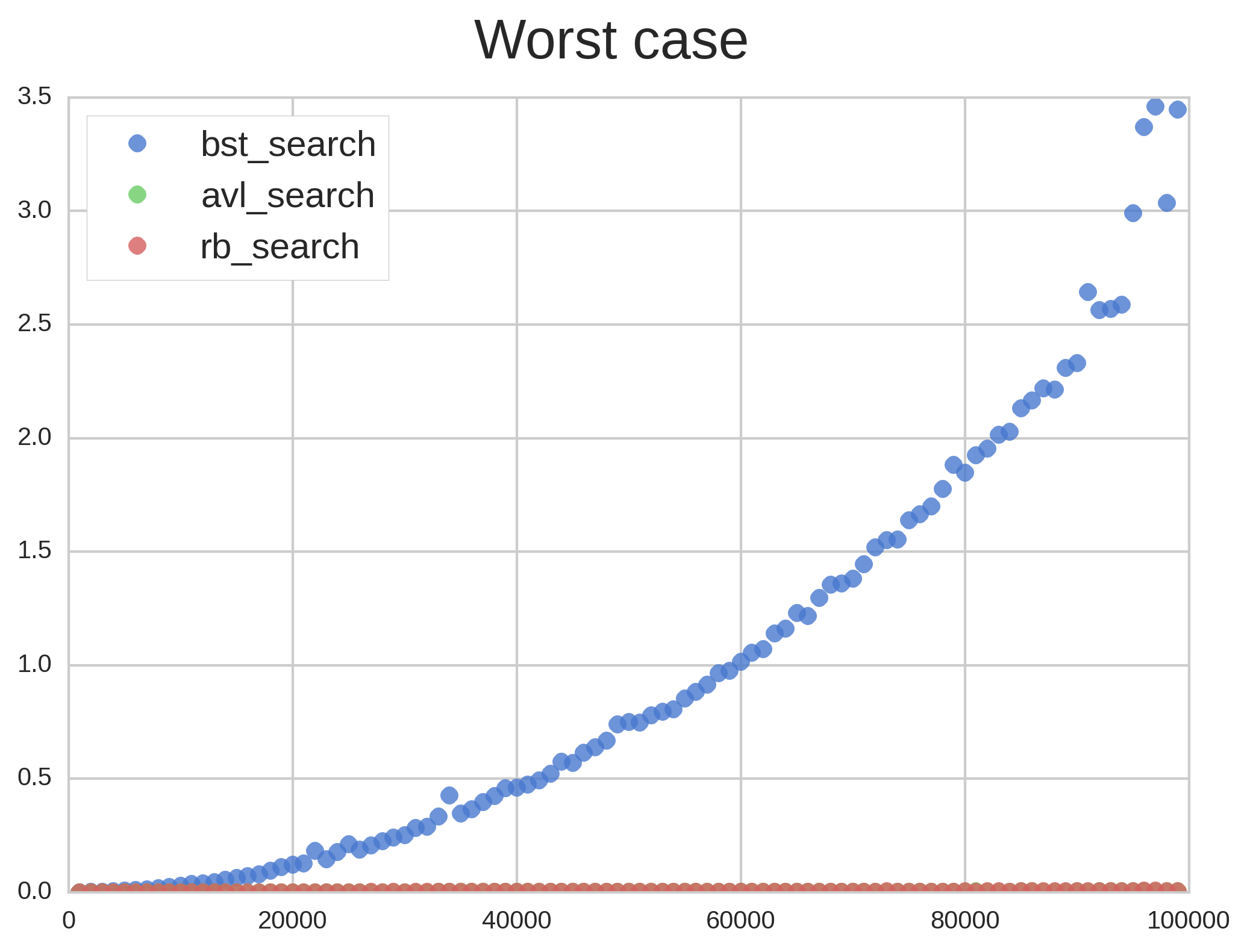
Figure 2
Figure 2 reminds us why self-balancing trees were invented. BST quickly degenerated into a $latex O(n)$-time linked list, which made the other two trees’ performance invisible. Let’s use a log plot to see how well R&B and AVL performed:
:————————-:|:————————-:
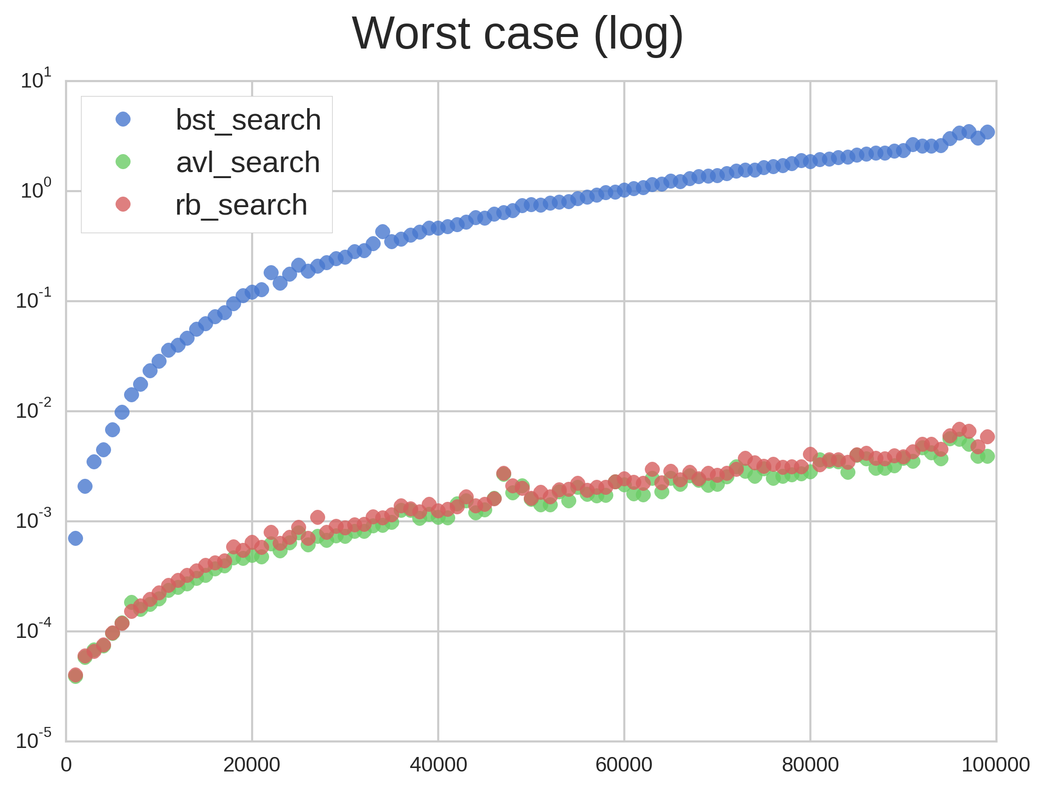
Figure 3
Figure 3 shows the same results as Figure 2 but with a logarithmic plot. As we can see, Red & Black and AVL trees performed nearly identically since both have worst-case $latex O(log(n))$ times. The difference in factors between AVL and RB isn’t really noticeable. AVL seems to have performed only infinitesimally better than RB, but the difference is most likely insignificant (statistically speaking).
The huge difference in performance between average and worst case are easily understood by looking at Figure 4. While BST height does increase more than the other trees’ height on the average case, they all have the same order of magnitude. Not on the worst case, though: BST height increases linearly while AVL and RB are clearly logarithmic.
:————————-:|:————————-:
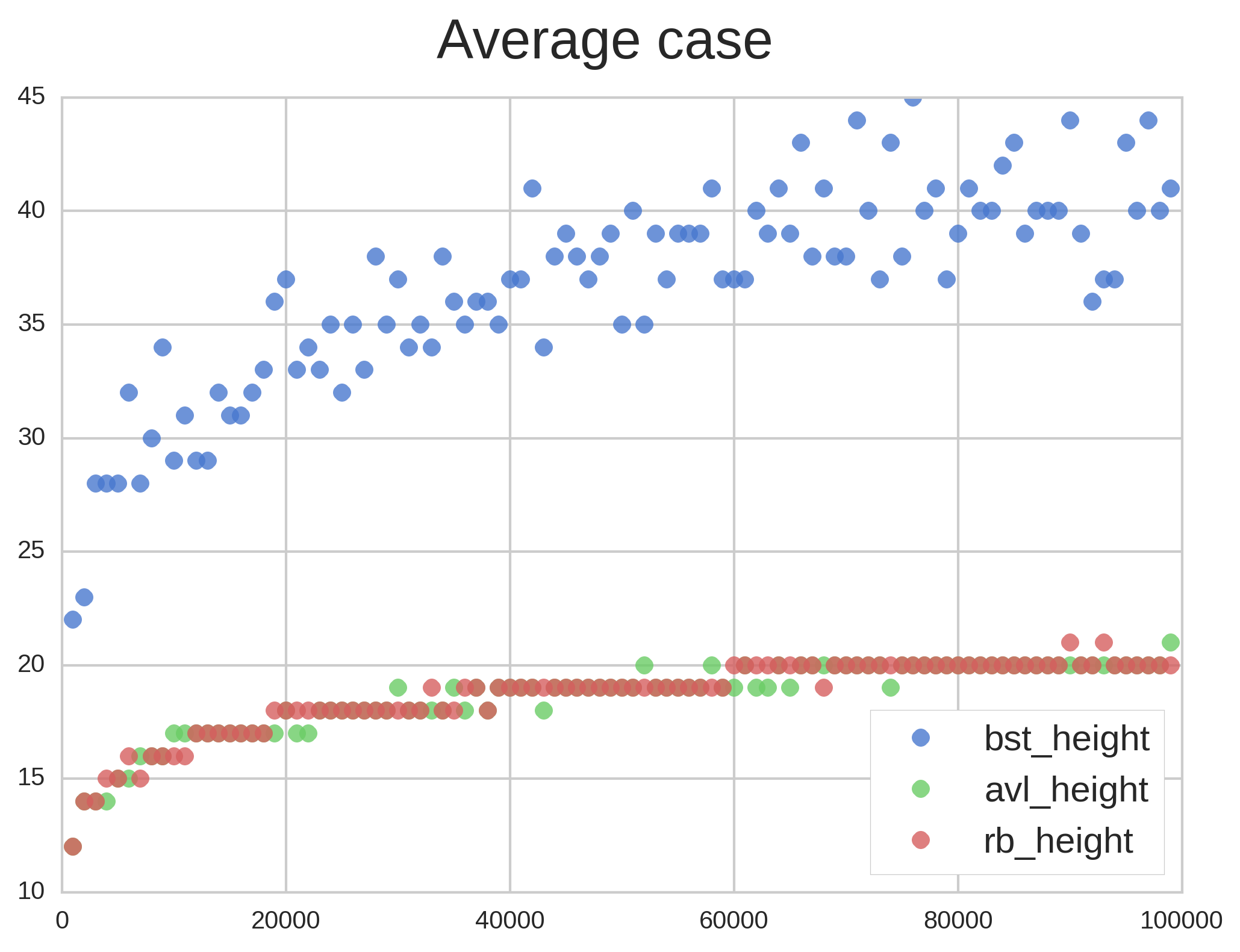
Figure 4
We are also able to notice the difference between AVL and Red-black factors in Figure 4’s right picture, where AVL’s height is consistently less than Red-black’s.
Figure 5 shows only Red-black and AVL heights. Note that they are close to the theoretical bounds, which suggests that our worst case is indeed a worst case. Take n = 80000 as an example: for the AVL tree we expect a height always smaller than $latex 1.44~log_{2}(80000) \approx 23.45$, while the observed was 20. For the Red-black tree, the upper bound is $latex log_{2}(n) \approx 32.57$, also close to the observed (30). Although these differences may seem big, they aren’t enough to significantly change observed search and insertion times (Figure 6). That’s what makes Big O so great!
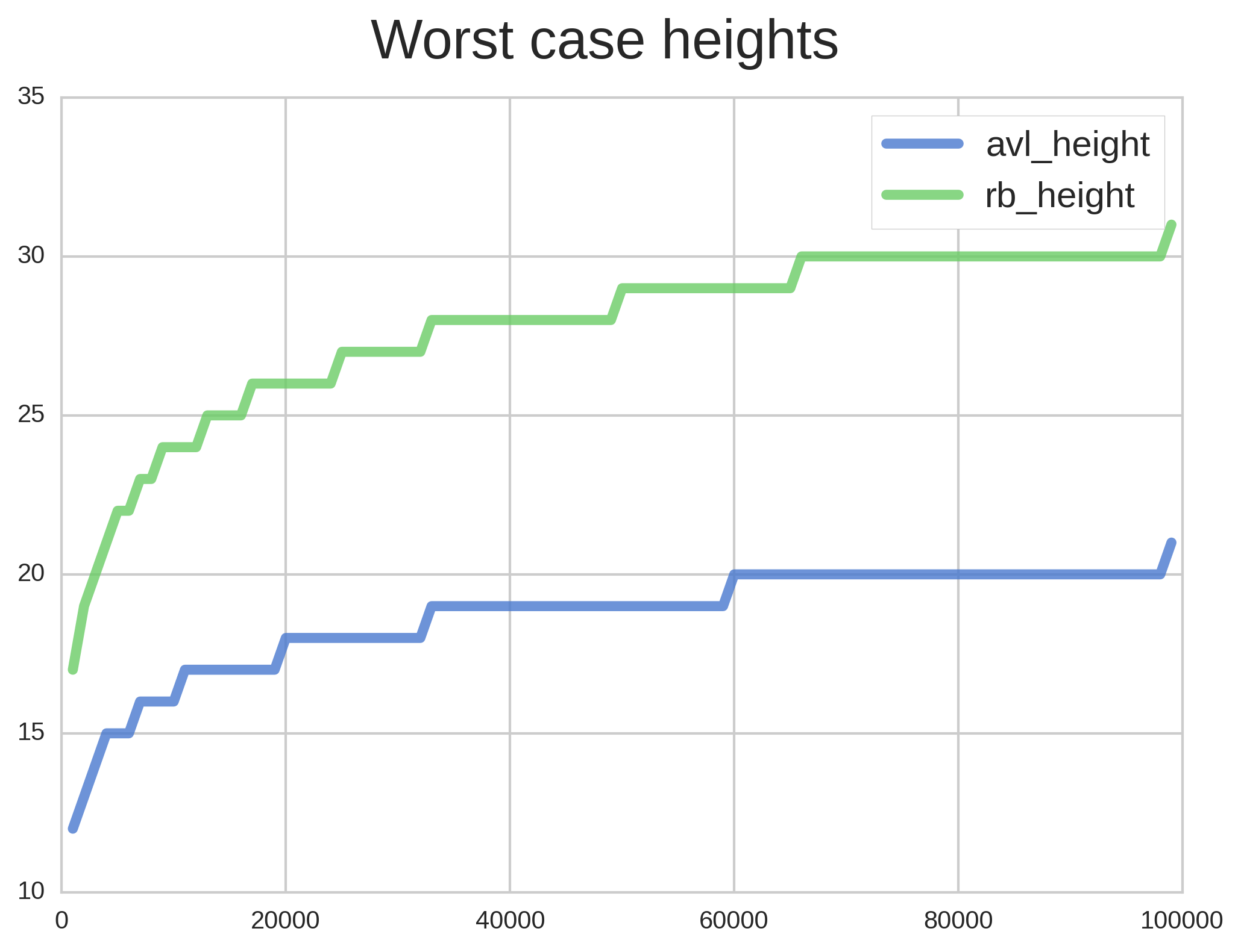
Figure 5
:————————-:|:————————-:
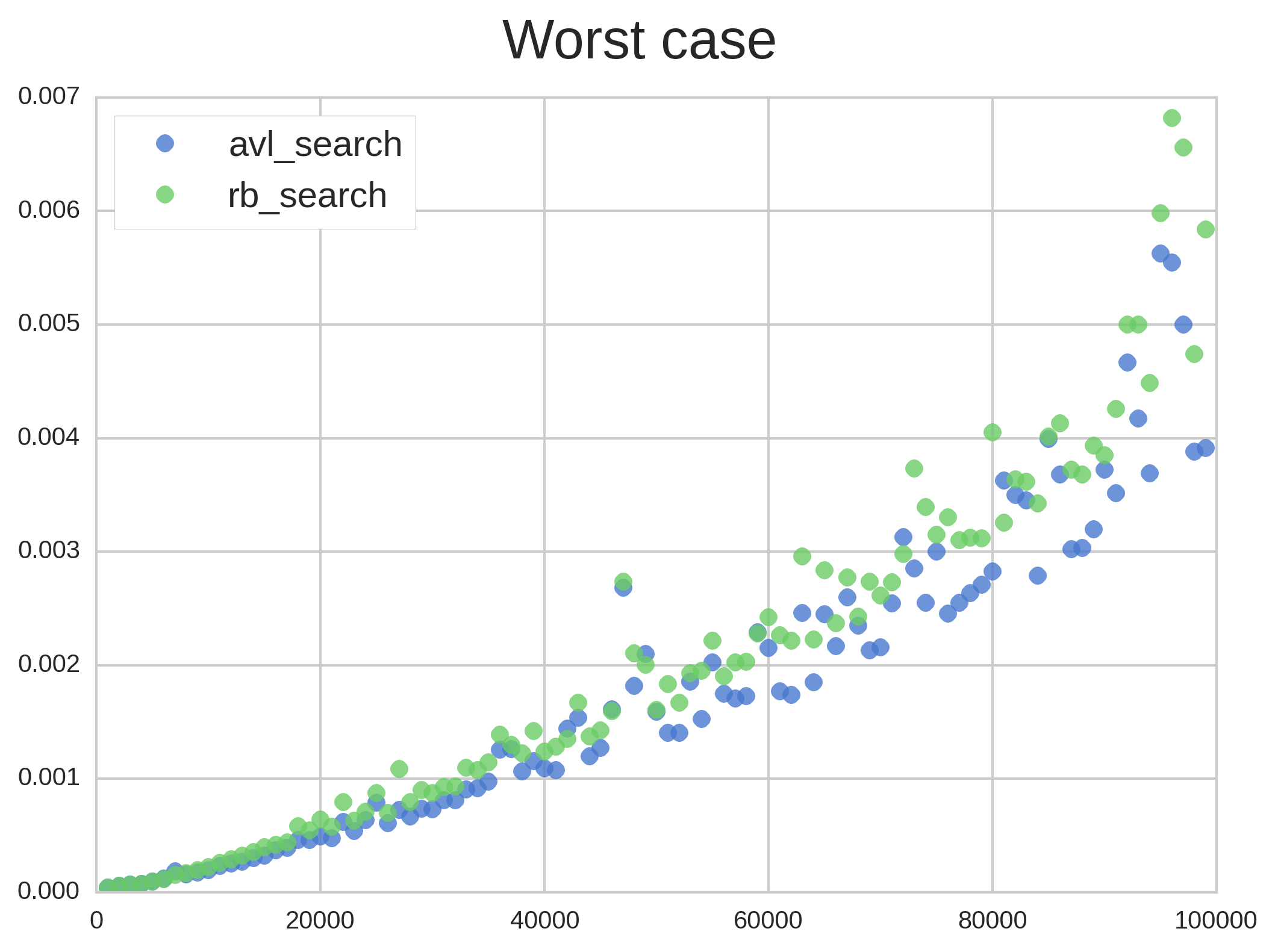
Figure 6
This concludes our analysis of self-balancing BSTs. As always, all the code used in this post can be found on Github. Charts were rendered with Matplotlib + Seaborn.