render(‘/image.*’, caption: ‘Bright green tree - Waikat’, src: ‘//upload.wikimedia.org/wikipedia/commons/thumb/f/f6/Bright_green_tree_-Waikato.jpg/512px-Bright_green_tree-Waikato.jpg)](http://commons.wikimedia.org/wiki/File%3ABright_green_tree-_Waikato.jpg)
We used trees to build the heap data structure before, but we didn’t bother with the theory behind trees, which are abstract and concrete data structures themselves. There’s a huge range of material to cover so I’ll split this in several posts.
In this first post we’ll cover the basic theory and implement a binary search tree (BST), which provides O(h) time search, insert and delete operations (h is the tree height). First, the basics:
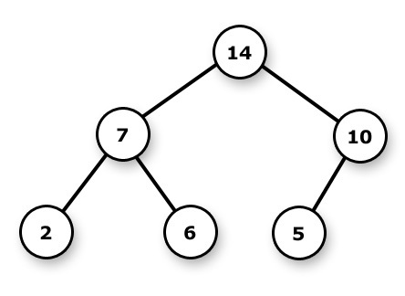
Trees are graphs with a few extra properties and interpretations/conventions. * Trees have height (longest branch length) and depth (distance to root). * The uppermost level consists of at most one node (the tree root). * All nodes may have children. * There are no edges other than parent-child edges.
Trees are classified according to some of those properties above and some others we’ll mention later. Most commonly, there is a constraint to the maximum number of children per node -e.g. the binary tree limits children to 2 per node. To build a BST, we’re going to need a working binary tree (BT) first. There are several ways to implement a BT. I chose a linked data structure:
typedef struct node
{
      void* data;
      struct node* parent;
      struct node* left_child;
      struct node* right_child;
} node;

typedef struct
{
      node* root;
      int order;
      int (*cmp) (void*, void*);
} binary_tree;
Together with their respective memory allocation functions (which I’ll omit for now), those two structs are enough to define a BT. Before we get into actually filling a tree with stuff, let’s assume we have a tree and take a look at tree traversal.
Traversing a tree means visiting all the nodes in the tree data structure. Whilst linear data structures (arrays, linked lists etc) have a default traversal order, trees do not. The traversal methods are classified according to the specific order in which the nodes are visited. Specifically, we are interested in breadth-first and depth-first traversals.
Depth-first searches (DFS) start at the (sub)tree root and “sinks” down until it reaches a leaf. Breadth-first searches (BFS) start at the root and exhaust all of its children before descending any further. Visiting in DFS can be done pre-order, in-order or post-order. The “order” refers to the specific time when we visit the root: before, after or in between visiting the sibling(s).
void dfs(node* n, void (*visit) (node*), int v_order)
{
      if (n!=NULL)
      {
            if (v_order == PRE_ORDER) visit(n);

            dfs(n->left_child, visit, v_order);

            if (v_order == IN_ORDER) visit(n);

            dfs(n->right_child, visit, v_order);

            if(v_order == POST_ORDER) visit(n);
      }
}
Now let’s take a look at binary search trees (BST). BSTs are binary trees with the following additional condition:
“Let x be a tree. If y is a node in the left subtree of x, then key[y] <= key[x]. If y is a node in the right subtree of x, then key[y] >= key[x].”
In other words, for every node in a BST (with unique elements), all values to the left are smaller and all values to the right are bigger than it. Note that this may appear similar to the heap property but is not the same at all: unlike with the heap, BST siblings and cousins are ordered in a specific way.
To preserve the BST property, we need to insert stuff in a specific order:
/**
 *  @brief Insertion
 *
 *  Starting from the root, we dive down through
 *  the children until we reach the node whose
 *  value is closest to the value of the node we
 *  want to insert.
 *
 *  @param [in] bt
 *  @param [in] n
 *  @return Return_Description
 */
void tree_insert(binary_tree* bt, node* n)
{
      node* cur = bt->root;
      node* prev = NULL;
      int goes_to = -1;

      while(cur!=NULL)
      {
            prev = cur;
            if ( (bt->order == ORD_ASC)
                  ? bt->cmp(cur->data, n->data) < 0
                  : bt->cmp(cur->data, n->data) > 0 )
            {
                  cur = cur->left_child;
                  goes_to = LEFT;
            }
            else
            {
                  cur = cur->right_child;
                  goes_to = RIGHT;
            }
      }

      if (prev != NULL)
      {
            n->parent = prev;
            if (goes_to == LEFT)          set_child(prev, n, LEFT);
            else if (goes_to == RIGHT)    set_child(prev, n, RIGHT);
            DBG("Node (#%d) inserted\n",*(int*)n->data);
      }
      else  // tree is empty, insert @ root
      {
            DBG("Node (#%d) set as ROOT\n",*(int*)n->data);
            bt->root = n;
      }
}
Starting at the root, we float down - moving left and right - until we reach the correct position for the node we’re inserting, always keeping track of the current node’s parent so it can be updated accordingly.
Together with a in-order DFS traversal, we can already do something useful with our BST tree: ordering a random set of values (integers in our case).
void depth_first(binary_tree* bt, void (*visit) (node*), int v_order)
{
      DBG("\nSTARTED DFS\n\n");
      dfs(bt->root, visit, v_order);
}

#ifdef _DEBUG
int main()
{
      binary_tree* bt = new_binary_tree(compare_integer, ORD_ASC);

      int ts = 10;

      srand(time(NULL));
      int i;

      for(i=0;i<ts;i++)
      {
            int* data = malloc(sizeof(int));
            *data = rand()%(ts*10);
            node* n = new_node((void*) data);
            tree_insert(bt, n);
      }

      depth_first(bt, visit, IN_ORDER);
}
#endif
Here’s a sample output:
C:\code\c\cstuff\data_structures>bt
New node (#46)
Node (#46) set as ROOT
New node (#14)
Node (#14) inserted
New node (#85)
Node (#85) inserted
New node (#43)
Node (#43) inserted
New node (#63)
Node (#63) inserted
New node (#55)
Node (#55) inserted
New node (#91)
Node (#91) inserted
New node (#60)
Node (#60) inserted
New node (#72)
Node (#72) inserted
New node (#8)
Node (#8) inserted

STARTED DFS

Visited node #8
Visited node #14
Visited node #43
Visited node #46
Visited node #55
Visited node #60
Visited node #63
Visited node #72
Visited node #85
Visited node #91
Several other operations commented with concise explanations and printable tests can be found at data_structures/binary_search_tree.c in the blog’s Github.
Next post we’ll (probably!) cover the AVL tree, which is another kind of binary search tree.