Posted in 2014

Trees - Part I

tre

render(‘/image.*’, caption: ‘Bright green tree - Waikat’, src: ‘//upload.wikimedia.org/wikipedia/commons/thumb/f/f6/Bright_green_tree_-Waikato.jpg/512px-Bright_green_tree-Waikato.jpg)](http://commons.wikimedia.org/wiki/File%3ABright_green_tree-_Waikato.jpg)

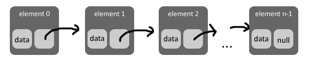
We used trees to build the heap data structure before, but we didn’t bother with the theory behind trees, which are abstract and concrete data structures themselves. There’s a huge range of material to cover so I’ll split this in several posts.

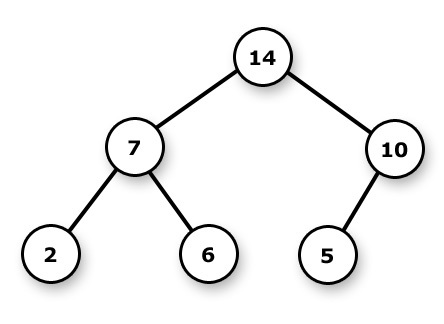
In this first post we’ll cover the basic theory and implement a binary search tree (BST), which provides O(h) time search, insert and delete operations (h is the tree height). First, the basics:

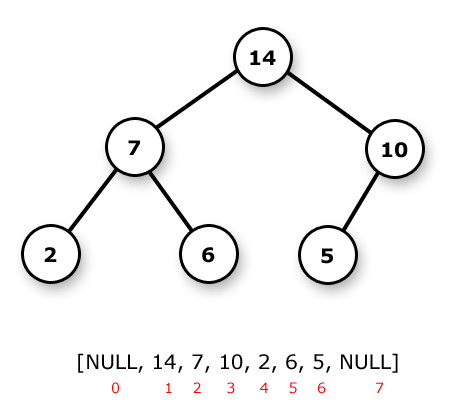
Trees are graphs with a few extra properties and interpretations/conventions. * Trees have height (longest branch length) and depth (distance to root). * The uppermost level consists of at most one node (the tree root). * All nodes may have children. * There are no edges other than parent-child edges.

Trees are classified according to some of those properties above and some others we’ll mention later. Most commonly, there is a constraint to the maximum number of children per node -e.g. the binary tree limits children to 2 per node.

Vector

Very simple Vector implementation with add, add_all, get and delete operations using arrays of void pointers.

The downside to this as compared to simply using an array is that here we have an array of pointers, which means the data will most likely be scattered over the memory, not coalesced.

Trees, Part II: AVL Tree

Masters classes started a few weeks ago, taking their toll on my productivity here. Sorry about that!

So we (pardon the nosism, but I think it sounds less egocentric than writing “I” all the time) hinted at AVL trees back on our Trees, Part I post. Specifically, we learned that:

a binary search tree (BST), provides O(h) time search, insert and delete operations (h is the tree height.

Linear time (O(h)) doesn’t sound very good - if h is close to n, we’ll have the same performance as a linked list. What if there were a way to bound the tree height to some sub-linear factor? As it turns out, there are several ways to do so, and the general idea of somehow keeping the tree height limited to a certain factor of the number of elements it holds is called height balancing. Ergo we’ll want to look into (height) balanced/self-balancing binary search trees **(BBST). **

                      Burger


                          M
                        .   .
                      .       .
                    .           .
                  .               .
                E .                 P .
              .     .                   .
            .         .                   .
          .             .                   .
      D .                 I                   Y
                        .
                      .
                    .
                  .
                F

AVL tree

Since binary search trees have at most two children, the best tree height (i.e. smallest) we can achieve is log2 n (n being the number of elements in the tree). There are several self-balancing BSTs developed over the years. It seems that up there in the US college professors tend to prefer the red-black tree when studying BBSTs, whilst over here AVL is preferred. In any case, AVL tree was the first BBST ever devised, so we’ll adopt it as our BBST model.

AVL trees (named after its two Soviet inventors Adelson-Velsky and Landis) use a series of rotations to keep the tree balanced. To keep track of when a certain subtree rooted at some node needs to be rotated, we maintain (or calculate) a balance factor variable for each node, which is the difference between the node’s left and right children’s heights, i.e.:

balance_factor(n) = n.left_child.height - n.right_child.height

Linked List

Here’s a very simple implementation of the linked list data structure.

A pointer to the head element is enough to define a linked list. Each element consists of one pointer to the subsequent element in the list and one pointer to the element’s data:

linkedlis

Heap & Priority Queues

Priority queues (PQs) are abstract data types that work just like regular stacks, but the popping order depends on each element’s priority instead of the sequence they were pushed onto the queue (FIFO or LIFO).

The naïve way of implementing a PQ consists of using an unsorted list or array and searching for the highest-priority element at each pop, which takes O(n) time. There are several more efficient implementations, of which the most usual is the heap.

Heaps are complete (i.e. all levels except possibly the last are filled) binary trees that work as PQs by maintaining the following property: children nodes always have a smaller priority than their parent, i.e. for any node A with children B and C, priority(B) < priority(A) && priority(C) < priority(A). Note that there is no assumed relation between siblings or cousins.

max-heap and corresponding array.

Each element of a heap has two pieces of information: a key and a value, hence we call them key-value (KV) pair. The key identifies the specific element, and the value determines the element’s priority within the heap. Heaps can be min-heaps (low value = high priority) or max-heaps (high value = high priority).

BurgerGFX - simple 2D graphics

sample code and outpu

Several times I find myself wanting to visualize something in 2D, but can’t bother to fire up OpenGL or other cumbersome API.

So I wrote a simple program which I called BurgerGFX, with 2 core functionalities: draw point and draw line. I find this to be quite enough for simple applications such as viewing a graph.

Setting up the drawing canvas, which I call burger, is simple: call create(width, height), which returns a pointer to the burger. Then simply call the draws, prints and cleans as needed.

Graph

Mathematically, a graph is a set of vertices and edges, thus a graph G is usually written as G(V,E). Besides linking vertices in the graph, edges can also carry a specific value which may be interpreted as cost, weight, distance etc.

graph viewed with BurgerGF

In computer science, we’re interested in the (abstract) data structure used to implement the graph mathematical concept. Let’s first discuss the basic elements in a graph - vertices and edges:

typedef struct vertex
{
 unsigned long id;
 int status;
 double x,y;
 void* data;
} vertex;

Vertices should be able to hold any kind of data, so we’ll just throw in a void pointer for that. Other than that we have an id, status (marked or unmarked - more on that later) and 2D coordinates so we can draw the vertices somewhere.

typedef struct edge
{
 vertex* from, *to;
 int cost;
} edge;

Edges consist of just pointers to the vertices they link and an optional value used as weight, distance, cost etc. Strictly speaking we could use a void pointer for that value as well, as long as we also defined a comparison function. But let’s save the hassle and just use an integer instead - most algorithms will be fine with that.

Shortest path, part I - Dijkstra's algorithm

Now that we have a way to represent graphs, we can discuss one of the most important problems in graph theory: the shortest path problem (SPP). More or less formally, we’ll define SPP as:

Given a weighted graph G(V,E), find the sequence P = {v0, v1, v2, …, v(n-1)}, vi ∈ V, from vertex V0 to vertex V(n-1), such that the list of edges EP = {(v0,v1), (v1,v2), … (v(n-2), v(n-1))} exists and the summation of costs of all elements e ∈ EP is the smallest possible.

In other words, find the less expensive (ergo “shortest”) path between two vertices.

The trivial solution is using BFS starting at vertex A and stopping when it reaches vertex B. However, BFS doesn’t look at the edge costs: it calculates the path with least edges, not the path with least total cost.

Although not necessarily the fastest, Dijkstra’s algorithm is probably the most popular way to solve the shortest path problem due to its simplicity and elegance. The algorithm relies heavily on priority queues, so make sure to take a look at that if you haven’t already.

Pseudocode

dist[from] = 0
for v : G
      if v != source
            dist[v] = infinity
      prev[v] = -1
      PQ.add(v, dist[v])
while PQ.hasNext()
      u = PQ.pop()
      for each neighbor v of u
            alt = dist[u] + length(u, v)
            if alt < dist[v]
                  dist[v] = alt
                  prev[v] = u
                  PQ.decrease_key(v,alt)
return prev

Doubly linked list

A doubly linked list is like our previously implemented Linked List, but instead of only having pointers to the next element, it also has pointers to the _previous _element:

610px-Doubly-linked-list.sv

This property makes the doubly linked list very useful as a base for other data structures such as the stack: having a previous pointer means we can quickly (O(1)) remove objects from the list’s tail, which would be impossible with a linked list.

We won’t discuss implementation since it so similar to a linked list. If anything implementation is even simpler than a linked list because of the previous pointer access.

Stack

Using our implementation of a doubly linked (DL) list, we can very simply build the most basic LIFO (last in, first out) data structure: the stack.

stac

Stacks have two basic operations: push and pop. Push pushes data onto the stack (i.e., end of the DL list) and pop pops data off the list’s tail, which is only possible because we can set the new tail as tail->prev, since we’re using a DL list, with previous pointers. Another useful function is peek, which returns a pointer to the stack’s top.

Mergesort

Mergesort is an important sorting algorithm when you don’t have efficient random memory access, since it doesn’t rely on that and has good time complexity - O(n logn) specifically.

As a typical divide-and-conquer algorithm, Mergesort has two steps: first it recursively splits the lists in two until each half is unitary, then it recursively mends back the lists until it reaches the original size.

But before we dive into the actual algorithm, we need to make some changes to the linked list algorithm we’ll be using.